Incrementality & measurement in the era of digital marketing

“Half the money I spend on advertising is wasted; the trouble is, I don’t know which half” once said John Wanamaker, the famous marketing pioneer. And almost two centuries later, the issue remains the same in modern-day marketing: measuring the true impact of a campaign remains an idealistic goal, a goal that marketing experts seldom reach.

At Numberly, we believe that incrementality measurement, especially through experimentation, is a solution that provides more reliable insights than the market’s standard (attribution measurement). However, incrementality is not perfect and has its drawbacks: the complexity of the experimentation process, and the access to the required data can make it difficult to conduct. That is why we take pride in the expertise we have developed in data collaboration, incrementality measurement methodology, and bias analysis to provide our customers with the best possible insights on their marketing campaigns.

The concept is pretty simple: when using attribution models, you introduce some uncertainty on what you measure. If someone makes a purchase right after being exposed to a campaign, this purchase is counted as a result of a campaign. So you never know how many of your exposed customers would have made a purchase anyway.
The generic solution is to define a group of customers, called the “Test group” or “Treatment group”, that you target with your marketing campaign. Then you compare their turnover to the turnover that would have been generated without your campaign. The difference is logically the uplift generated by your campaign on your turnover.

Of course, “the turnover that would have been generated without your campaign” is the tricky part. Ideally, we want to have a group of customers similar to the test group, which we will call the “Control” or “Holdout” group, and measure their turnover in the same period as the test group, but without exposing them to our campaign. This should give us the amount we want to compare to. But we will see that creating this group is more complicated than what we think.

This campaign was a failure (the treatment and control group are absolutely identical), but the exposure bias can lead many people to believe it was a success.

Having a similar group is a complex task that mixes marketing & mathematical expertise. One solution that works in most cases is to divide your customers into two groups randomly. The more customers you have, the more likely you are to obtain two similar groups thanks to randomness.

a. Creation of the populations

From what we’ve learned by now, we know that the only option left is to compare two identical populations. One solution would be to make sure that you can isolate such populations, by testing equal distribution according to gender, age, socio-economical value, CLV, purchase behavior, etc. This is a viable option in some cases, but it has some limitations:

• You don’t always know what is the determining factor in a population: do we want to correct our population in terms of gender, age, visits on site, purchase, geography, all of the above? What if there is a criterion you don’t know about such as a specific interest that is determining to compare populations?
• You get less precise results than with inherently similar populations.

This methodology will be detailed in part 4, as this allows us to get incremental measurements after a campaign has already been conducted, which is a frequent business case for our clients.

This is why the best method when possible is to create your test and your control group prior to your campaign and assign at random every individual to one group. Statistical law guarantees you that with enough customers in your audience (almost always reached in a real marketing use case), you will almost always get two identical sets.

b. Compare what’s comparable

Whatever method you use to create your two populations, it is necessary to control that they have similar purchase behaviors before your campaign. This verification is needed to confirm that the difference you observe after the campaign is purely due to your marketing incremental effect.

c. Take into account the dilution

Now that we have our proper set of experimentation, conducted our campaigns, and got our results, it’s time to dive into statistics and make sure we understand what effect is measured. For that, we must introduce some useful terminology from the medical field.

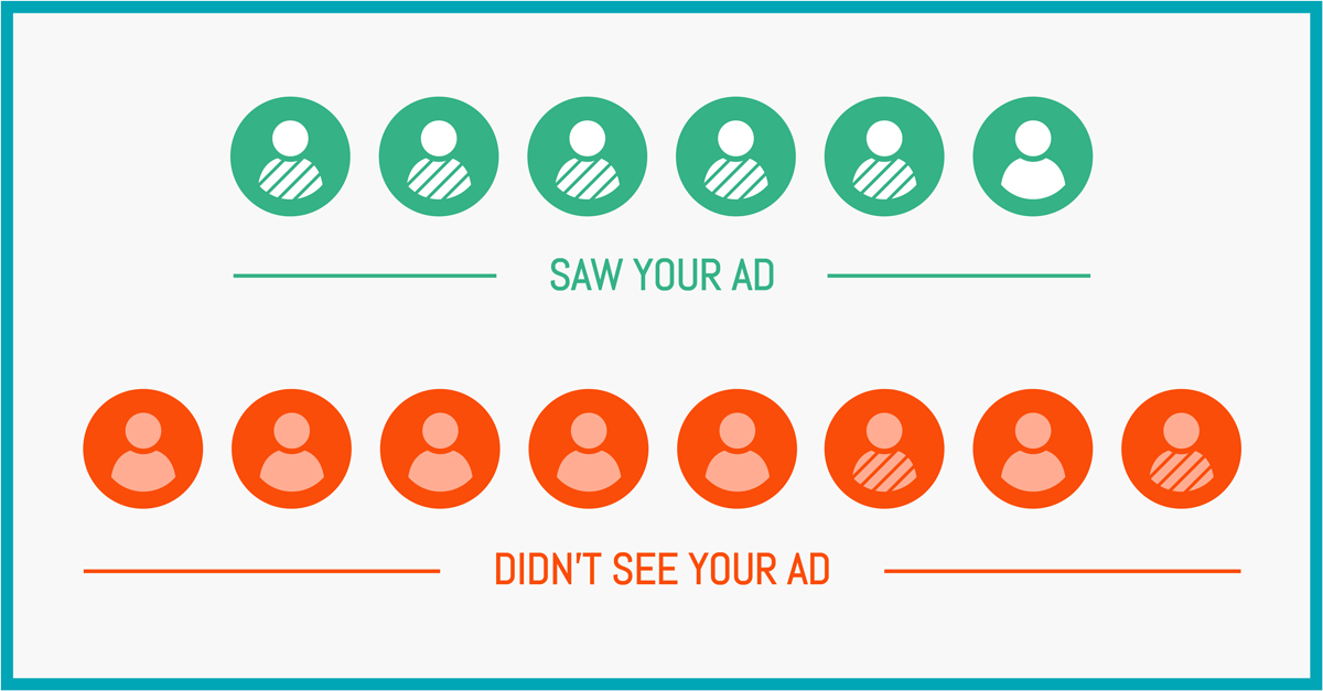
In pharmaceutical studies, biases can intervene while trying to measure the true effect of a given drug. The reader is probably familiar with the placebo effect for example: taking a drug, even ineffective, can have a significant psychological (and then physical) effect. Another less famous phenomenon is the possibility for the patient to refuse medication, or pretend to follow a treatment while actually not using the drugs. This behavior can be caused by some pathology or could be the patient’s own choice. If the placebo effect is not that relevant to our marketing study, the latter is crucial: indeed, just like people can refuse to take a pill even though they received the true treatment, people can avoid exposition to an ad even though they are in the targeted test group (for example, if the person is on holiday during the campaign and no impression is available).
We then distinguish two measured effects:

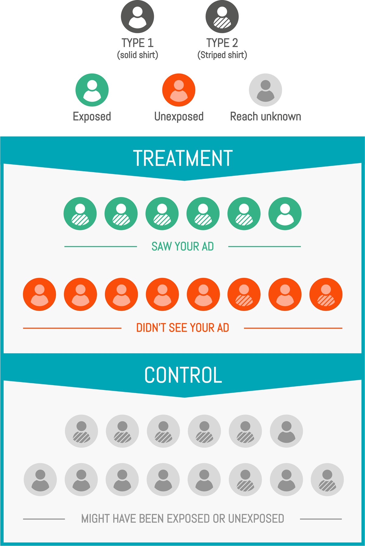
• Intent-to-treat (ITT): This represents how the prescription of the drug affects the health of a patient, without knowing if they will actually take it or not.
• Local Average Treatment Effect (LATE): This captures the actual effect of taking the drug on the health of a patient.

In our case, we can assimilate the ITT effect to our targeting: what is the incremental effect of targeting a population? The LATE is the exposure effect: what is the incremental effect on those who saw our ad?
The ITT is the most global and least detailed indicator: it combines the LATE effect and the probability of exposure in one.
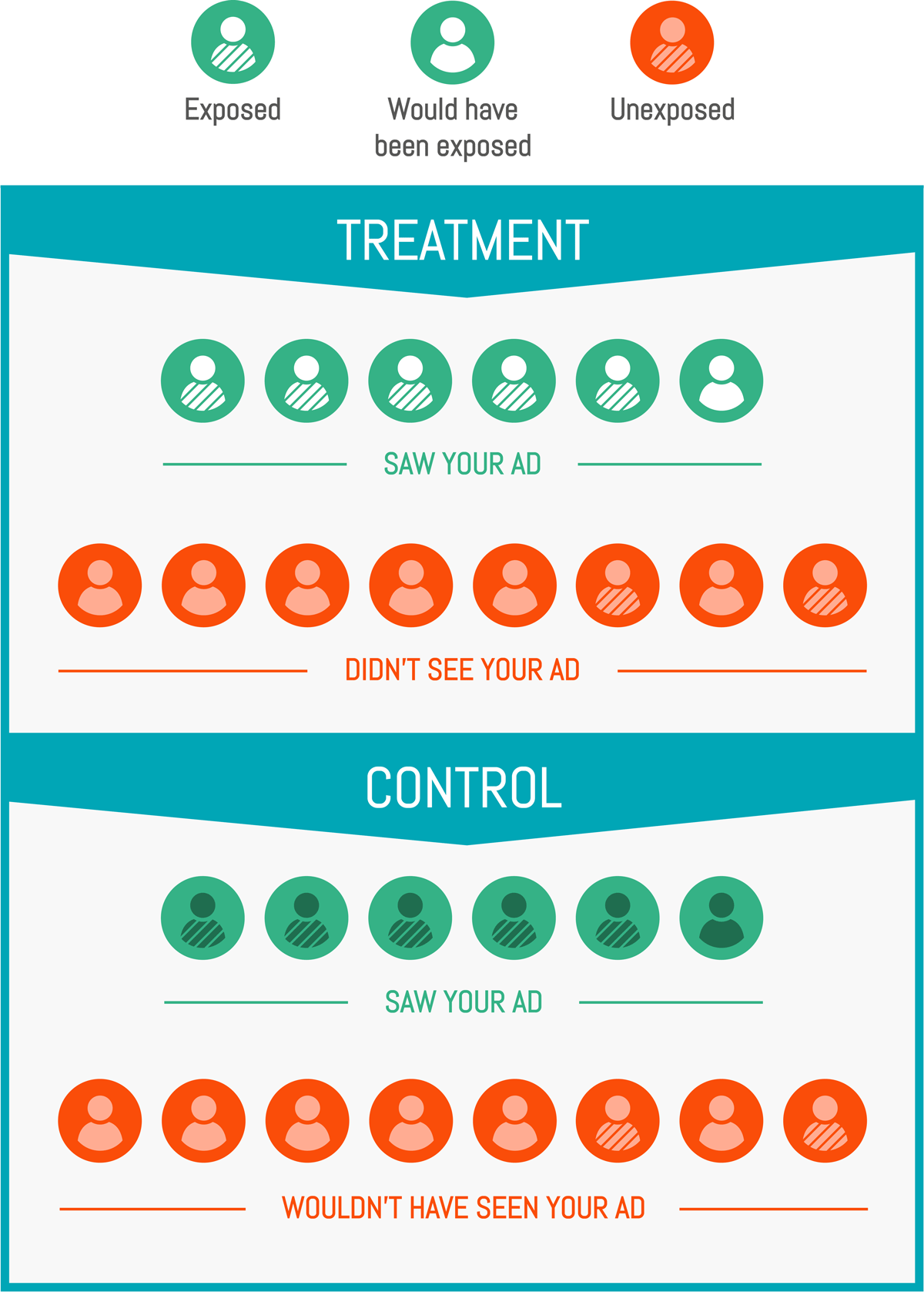
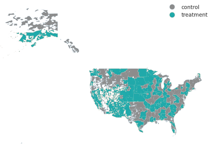
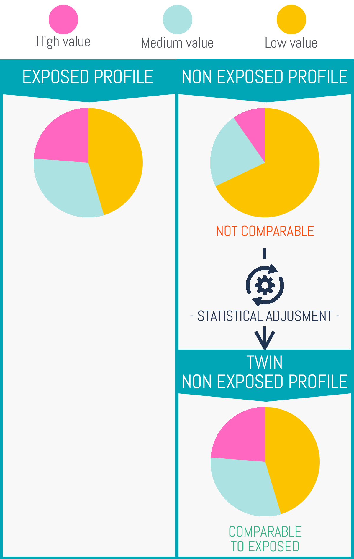
It is easy to measure: you simply need to compare your test and control group. The LATE is more tricky: you cannot compare exposed to unexposed customers because, as we saw earlier, your exposable customers (those that are easy to reach, as opt-in for CRM programs or internet natives for media audiences) are inherently better than the rest.

For example, let’s take a mailing campaign that generates a 10% increase in sales.
You know that people who always open emails from your brand are your engaged customers. Let’s assume they generate 50% more sales in general than your regular customers.
Those customers will generate (1+10%)*(1+50%) = 65% more sales than the others. But you will only be able to measure that 65% (cumulative effect of ad + bias on engaged customers), and what you want to measure is the 10% increase in sales.

This is why we take into account the exposure rate, pollution (customers in the control group that were exposed unintentionally), technical limitations, and several parameters of the campaign (total and frequency of exposure, visibility, duration) to compute the actual effect estimated for the campaign, our Local Average Treatment Effect.

This method is less precise than experimental ones, plus the methodology requires to have enough data on the customers to be able to build a relevant twin group. However, it has the advantage of requiring no setup and no holdout group (which means, no impact on the diffusion).

Measurement in marketing is a much more complicated process than it looks, requiring a deep understanding of statistics, marketing biases and insights, experience from comparable projects, and technical limitations.

But measuring our incremental effect is only the first step towards building an action plan. The work of the analyst begins after obtaining that first measure: what subpopulations are the most interesting? What is our seasonal effect? (meaning: would our campaign have the same impact in summer or winter?) What insights can I get from this measurement to better understand my customers and how to reach them? How can I optimize my campaign parameters, or combine different levers such as media and emails to create the best possible synergy?